1What Real-Time Spectrum Analysis Is
A spectrum analyzer answers one question: what energy is present, and at which frequencies. For decades the standard way to answer it was to sweep. A tuned receiver walks across the band, dwells briefly at each step, measures the power, then moves on. That works beautifully when the signals you care about sit still and stay on. It fails the moment a signal turns on and off faster than the sweep can reach it.
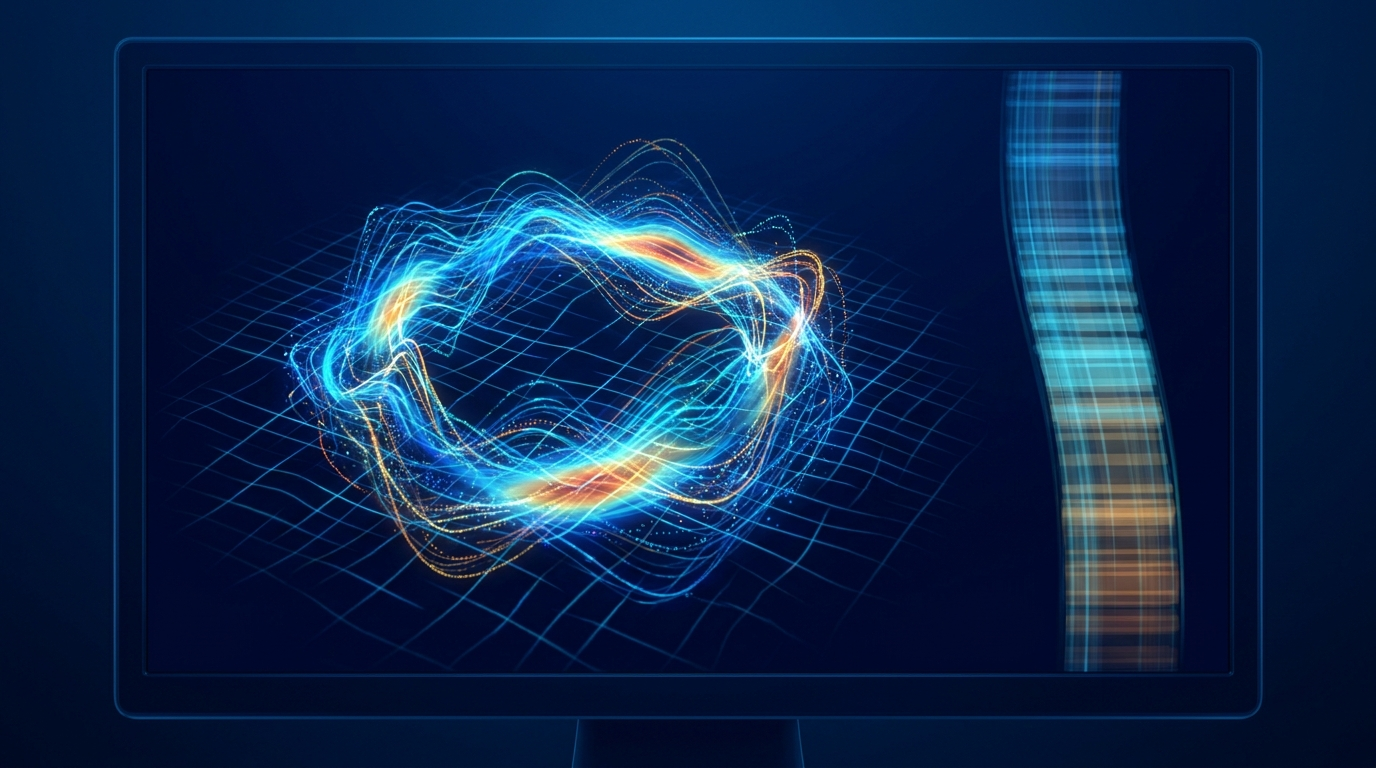
Real-time spectrum analysis takes a different stance. Instead of visiting frequencies one at a time, it captures a wide block of spectrum all at once and keeps capturing it without pause. The instrument transforms a continuous stream of samples into a continuous stream of spectra, so a burst that lasts only microseconds still lands inside a measurement window.
This matters more every year. The spectrum is crowded. Frequency-hopping radios change channels thousands of times a second, radar pulses come and go in microseconds, and interference often shows up as a short spit of energy that never appears twice in the same place. Agile, intermittent, and overlapping signals are now the norm. A swept analyzer can spend its whole sweep looking at the wrong frequency at the wrong instant. A real-time analyzer is built so that does not happen.
2Three Architectures, Compared
It helps to see where real-time analysis sits among the instruments engineers actually reach for. Three architectures dominate, and each makes a different trade.
Swept / superheterodyne
The classic design. A local oscillator tunes the receiver across the span while a narrow filter measures power at each step. The strength is reach and resolution: you can sweep enormous spans and resolve very close tones with a narrow resolution bandwidth. The trade is time. The analyzer only ever looks at one slice at a time, so anything happening elsewhere during that slice is invisible. For stable carriers and slow drift it remains an excellent, economical tool.
Vector signal analyzer (VSA)
A VSA digitizes a slice of spectrum and preserves both magnitude and phase, which lets it demodulate. It will hand you constellation diagrams, error vector magnitude, and the inner structure of a modulated signal. The strength is depth of insight into a known signal. The trade is that a VSA is built to dissect a signal you already expect, not to stand watch over a whole band waiting for something unexpected to flash by.
Real-time (RTSA)
An RTSA also digitizes a wide slice, but it processes that slice continuously and without gaps. Its strength is certainty of capture: if a signal occurs inside the analysis bandwidth, the instrument is guaranteed to see it down to a known minimum duration. The trade is that real-time bandwidth is finite, so you watch a defined window rather than the entire span at full speed. Many modern analyzers blend the three, sweeping for wide coverage and switching to real-time inside the band that demands it.
3How an RTSA Works
The mechanism is easier to follow than the marketing around it. Three things happen, and they happen at once.
First, the analyzer digitizes a wide block of spectrum. A downconverter places the band of interest at an intermediate frequency, and a fast analog-to-digital converter samples it as in-phase and quadrature data. The width of this captured block is the real-time bandwidth, and it sets the largest window the instrument can watch all at once.
Second, the analyzer runs a Fast Fourier Transform on that sample stream to turn time-domain samples into a spectrum. The trick that makes the analysis real-time is that the FFTs never stop and they overlap. Rather than process one block, pause, then grab the next, the engine slides the FFT window forward by a fraction of its length and transforms again. Overlapping windows mean that an event near the edge of one window also sits comfortably inside the next, so no signal is penalized for arriving at an awkward moment.
Third, the result is gap-free coverage. Spectra arrive in a contiguous train, each one a fresh photograph of the whole real-time band. Stack enough of them per second and the picture is effectively a movie of the spectrum with no missing frames. That contiguity is the entire point, and it is what the next section quantifies.
4Probability of Intercept
If a real-time analyzer makes one promise, it is this: a signal of at least a certain duration that falls inside the analysis bandwidth will be captured with full confidence. That guaranteed minimum duration is the probability of intercept, or POI. It is the headline spec because it answers the question a swept analyzer cannot: how brief can an event be and still be certain to show up.
Two things drive POI. The first is the FFT rate, meaning how many transforms the engine completes each second. The faster the spectra arrive, the shorter the event that still lands inside one of them. The second is window overlap. When successive FFT windows overlap heavily, a signal cannot hide in a transition gap, and a shorter event is still seen at something close to its true level. Push the rate up and the overlap up, and POI comes down.
One distinction trips up newcomers, so it is worth stating plainly. There is a difference between POI for detection and POI for amplitude accuracy. Detection POI is the shortest event the analyzer will reliably notice at all, often quoted at a modest level below the true amplitude. Amplitude POI is the longer minimum needed for the measured level to sit within a tight tolerance, frequently within a fraction of a decibel, of the real value. A vendor can advertise a very small POI and still be honest, as long as you read which one it is. Detecting a 5 microsecond pulse is one claim. Measuring its power within half a decibel is a stronger one.
5RBW, Span, and Windowing
Three settings shape every spectrum, and they pull against each other. Understanding the tension is most of the skill.
Resolution bandwidth (RBW) is how finely the analyzer can separate two close tones. A narrow RBW resolves detail but takes longer to compute and reduces how fast spectra can arrive. Span is how wide a frequency range you display. A wide span shows more of the world at once but, for a given FFT size, spreads the resolution thinner. The link between them is the FFT itself: the number of points and the captured bandwidth together fix the bin spacing, and the bin spacing sets the achievable RBW.
Windowing is the third lever. Before each FFT, the sample block is multiplied by a window function that tapers its edges to zero. Without it, the abrupt block boundaries smear energy across the spectrum, an effect called spectral leakage, and small signals near large ones disappear into the skirts. The choice of window trades main-lobe width against side-lobe height. A flat-top window gives excellent amplitude accuracy at the cost of frequency resolution, while a window like Hann or Blackman favors separating nearby tones. There is no universally correct window. There is only the right window for what you are trying to see.
6Density and Persistence Displays
Once spectra arrive thousands of times a second, a normal trace cannot keep up. Drawing one line per spectrum either flickers uselessly or, with averaging, erases the brief events you bought the analyzer to find. The answer is the density, or persistence, display.
Instead of plotting a single trace, the analyzer accumulates many spectra into a two-dimensional histogram. The horizontal axis is frequency, the vertical axis is amplitude, and color encodes how often each point in that grid was hit. A signal that is present nearly all the time burns in as a hot, saturated color. A signal that flashes for a microsecond once in a while paints a faint, cool wash. The display turns frequency of occurrence into something you can read at a glance.
The payoff is separation. A weak, intermittent emitter sitting underneath a strong, steady carrier is nearly impossible to see on a single trace. On a density display the two paint in different colors because they occur with different frequencies, and the eye picks them apart immediately. Bright means persistent, dim means rare, and structure in the color tells you the duty cycle of everything sharing that band.
7Triggering in the Frequency Domain
Catching an event is one thing. Catching the right event, and only that one, is another. Time-domain triggers fire on a level crossing, which is fine for a single channel but useless when the thing you want to isolate is defined by where it sits in frequency, not how loud it is overall.
The frequency-mask trigger solves this. You draw a mask, an outline across the span that describes the spectrum you expect to see. The analyzer compares every incoming spectrum against the mask in real time and triggers the instant any point crosses it. Set the mask just above a clean band and the analyzer sits quietly until an interferer pokes through, then captures exactly that moment with pre-trigger and post-trigger history around it. Set it to outline a known channel and you can trigger only on energy that appears where nothing should be. The mask turns "alert me when something unexpected happens at this frequency" into a single, automatic condition, which is precisely what intermittent-signal hunting demands.
8The Specifications That Matter
When you compare analyzers, a handful of numbers carry most of the weight. Read them together, because each one constrains the others.
| Specification | What it tells you |
|---|---|
| Real-time bandwidth | The widest contiguous block the instrument can watch gap-free at once. The single most important number for catching wideband or agile events. |
| Probability of intercept (POI) | The shortest event guaranteed to be captured. Confirm whether the figure is for detection or for amplitude accuracy. |
| DANL | Displayed average noise level, the floor beneath which signals vanish. It sets your sensitivity to weak emitters. |
| Dynamic range | The span between the largest and smallest signals measurable at the same time, so a strong carrier does not mask a weak neighbor. |
| Max FFTs per second | How many spectra the engine produces each second. It drives POI and how faithfully a density display reconstructs fast activity. |
A wide real-time bandwidth with a slow FFT rate still leaves brief events at risk. A blazing FFT rate over a narrow band cannot watch much of the spectrum at once. Strong sensitivity is wasted if the dynamic range lets a loud signal swamp the quiet one beside it. Judge the set as a whole, against the signals you actually expect to chase.
9Where It Gets Used
Real-time analysis earns its keep anywhere signals are brief, agile, or hidden in a crowd: spectrum monitoring and interference hunting, electronic warfare and signals intelligence, RF geolocation, drone and counter-drone detection, 5G and emerging 6G validation, radar and aerospace test, and EMI pre-compliance. Each has its own workflow, and the BNC application briefs walk through them in detail. Start with Spectrum Monitoring, EW & SIGINT, Drone Spectrum Monitoring, and RF Geolocation & Mapping.
10How the ICX-FieldHawk Line Implements It
The Berkeley Nucleonics ICX-FieldHawk family puts real-time analysis in your hand and in the field. The line covers 9 kHz to 40 GHz with 100 MHz of real-time bandwidth, enough to watch a wide block of spectrum gap-free and catch the brief, hopping, and intermittent signals described throughout this guide.
The analysis engine is SpecICX-gen3, which drives the continuous overlapping FFTs, the density and persistence display, and the frequency-mask trigger as a single workflow rather than a stack of bolt-on options. The same engine runs across three form factors so the measurement does not change when the deployment does. The handheld unit is built for walk-and-find work, the rugged ICX-FieldHawk-R stands up to harsh field and vehicle environments, and the USB ICX-FieldHawk-U turns a laptop or an embedded host into a full real-time analyzer for benches, racks, and remote sensors. Pair any of them with the ANT-100G directional antenna to turn detection into a bearing.
To talk through real-time bandwidth, POI, and the right form factor for your mission, contact Berkeley Nucleonics at 800-234-7858 or info@berkeleynucleonics.com.
For a quick question, chat with an engineer at berkeleynucleonics.com.