Chapter 8: Performance Tips

Straightforward power measurements under good conditions are usually not a challenge. Hook up a power meter and read the result. Many application-related issues can make the process more challenging, however. This chapter covers three topics: reducing measurement noise, optimizing ATE performance, and statistical techniques for amplifier testing.

8.1 Reducing Measurement Noise

Power measurements often span a wide dynamic range, and sensors can be challenged at both extremes. The top of the range usually has hard limits: average and peak power must remain within a safe (for the sensor) and calibrated range to be measured accurately. The lower end of the range is harder to define.

All measurements are made in the presence of noise. It is part of every electrical measurement, including RF power. Unless the amplitude of the signal is considerably greater than the noise amplitude, the noise adds to the measured signal and produces measurement uncertainty (see Chapter 9).

One convenient aspect of noise is that it is random. Power measurement noise is fairly wideband and roughly white, meaning constant power per hertz. If the bandwidth is halved, so is the average noise power. When the noise bandwidth exceeds the bandwidth of the signal to be measured, filtering the noise bandwidth reduces the total noise power.

CW signals represent the extreme case. The bandwidth of a CW signal is effectively 0 Hz, so it is possible to filter the signal and noise together to sub-1 Hz bandwidth without affecting accuracy. Most power meters provide an averaging filter that averages a number of readings over a defined time interval to yield a filtered result. Increasing the averaging time reduces the measurement noise at the expense of settling time when the signal level changes.

Other types of noise are present besides Gaussian noise, which causes increased filtering to reach a point of diminishing returns. A one-second filter time is generally appropriate for -60 dBm with a CW diode sensor. Increasing the filter to ten seconds will not reduce noise by a factor of ten and so will not allow the same accuracy at -70 dBm.

Most CW and average power meters include an auto-filter setting, in which the instrument chooses the filter time constant based on the measured power level. This can cause extended settling times when the level changes. If you know the expected power level, set the filter manually for best performance.

The averaging filter of most CW and average power meters, and peak power meters operating in continuous, free-run, or modulated mode, is most often a sliding-window filter. Power readings happen at a relatively fast rate and are averaged together as needed. The filtered power reading at any time is the average of the last N samples, where N is the filter time divided by the internal acquisition rate. Unweighted averages are most common, but other weightings are sometimes used to accommodate fluctuating signals such as pulse waveforms. By continuously adding new samples and discarding old ones, the filter output is recomputed and updated at the acquisition rate.

When measuring a wideband signal with a peak power meter, filtering noise becomes harder. Peak power meters often need to maintain measurement bandwidths of tens of MHz or more. It is not possible to apply filters with millisecond or second time constants without also filtering out desirable signal characteristics.

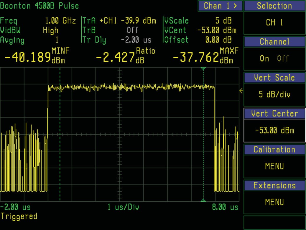
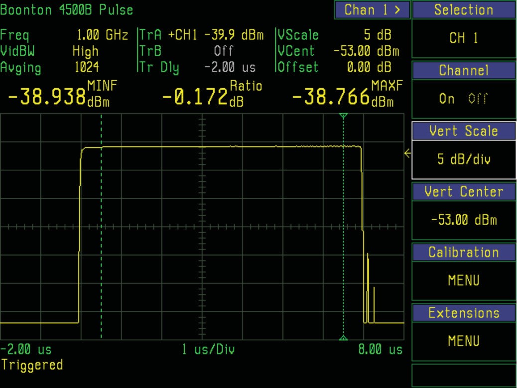
Take advantage of the redundancy of repetitive signals. Any periodic waveform can be synchronously filtered by averaging together multiple periods. As long as the individual periods or waveform events align closely in time, hundreds or thousands of cycles can be averaged together to produce a filtered waveform with significantly less visible noise and no degradation of the waveform's amplitude or profile. The result on a low-level (-39 dBm) pulse is dramatic. With no averaging, peak-to-peak measurement noise might be 2.4 dB. With 1024 averages, peak-to-peak noise during the pulse drops below 0.2 dB, and the noise floor moves down from -53 dBm to below -70 dBm.

Synchronous waveform averaging is often called "trace averaging" or simply "averaging" in peak power meters operating in triggered (pulse) mode. Sometimes the term "video averaging" is used, since it is familiar to spectrum analyzer users. This can be confusing in power meters.

The source of confusion is that some peak power meters offer an additional method for reducing noise. They reduce the video bandwidth of the sensor or meter input circuitry. This technique does not introduce errors as long as the video bandwidth of the measurement remains above the video bandwidth of the signal. In most cases, this bandwidth reduction offers only a modest reduction in noise, but it can make the difference between a signal that can and cannot be measured. It can be used in conjunction with filtering or averaging.

Another technique is simply to sample faster. If the meter is already sampling at or above Nyquist rate, this method will not yield significant improvement. If it is undersampling and has excess bandwidth, a faster sample rate tends to filter the noise without affecting the signal.

8.2 Optimizing ATE Performance

Modern peak power meters typically include high-speed connectivity (GPIB, LAN, USB) for remote control by a PC or system controller, integrating into automated test equipment (ATE) systems. This functionality extends instrument capabilities far beyond manual front-panel operation. Other devices combine with the power meter to provide a centralized location to control them and to collect and display data from multiple instruments.

The glue that ties instruments to a PC consists of a PC I/O interface such as the VISA library. VISA is short for VXIplug&play Systems Alliance, now part of the IVI Foundation. VISA lets the physical interface on the PC be its built-in serial, Ethernet LAN, or USB interface, a PCI-based GPIB card, a USB-to-GPIB cable, or a combination. The library includes the low-level drivers and functions required to use any of these interfaces for instrument control. The result is a portable, bus-independent programming model that frees the developer from implementing a low-level communication channel for each instrument and bus.

The developer chooses a development environment to create the automation software. The .NET IDE allows Visual Basic, C#, or C++ for code development. Iconic programming environments such as Agilent VEE or National Instruments LabVIEW let users create automation applications without extensive programming experience. Add-on libraries, utilities, and example programs make it easier for the non-programmer engineer to develop automation software for a specific application. Modern Berkeley Nucleonics drivers ship for Python, MATLAB, LabVIEW, and C/C++ on Windows, Linux, and macOS.

Instrument-to-host communication. Most instruments today adhere to the SCPI (Standard Commands for Programmable Instruments) software standard, which defines a common interface language. SCPI commands are ASCII text messages in a defined syntax and can be implemented in any PC host programming environment. Conformance means instruments with similar functions accept the same commands, minimizing or eliminating software changes when instruments are swapped.

All SCPI commands are sent as ASCII text strings, but measurement data returned by an instrument can be transferred either as ASCII (default) or in binary format. Binary is more compact. It is the most efficient method when both host and instrument use IEEE floating-point format, for three reasons. First, the binary-to-ASCII conversion on the instrument side is eliminated. Second, the ASCII-to-binary conversion on the host side is eliminated. Third, the number of bytes per value is reduced because of more efficient packing and the elimination of delimiters.

The default ASCII transfer mode is simplest to implement, since formatting is performed transparently by the VISA library. ASCII is also simplest for troubleshooting, because bus transactions can be monitored and logged using readily available tools. When reduced I/O traffic or transfer speed becomes an issue, binary transfer can improve system efficiency with a little more programming effort.

Why automate. Several reasons justify the effort.

• It provides consistency by eliminating possible errors from front-panel manual operation.
• Timing of system events and measurements can be made totally consistent.
• Higher throughput provides either reduced test time or the ability to collect more data in the same time.
• Automation facilitates large-volume production testing where test time and accuracy are paramount.
• Collecting results from multiple devices for processing and display on the PC enables information presentations beyond the capability of any single stand-alone device.
• Instruments can acquire data at a rate faster than their display update rate. PC control bypasses the display to take advantage of acquisition speed.
• Recording and archiving measurement results for QA or regulatory purposes is simpler.

Historically, RF power measurement in ATE systems was performed via a query-response protocol. ASCII command and data transfer were used in both directions, either via SCPI or proprietary protocols. Recent advances in power measurement, coupled with increased user requirements, have made it necessary to examine newer solutions for system throughput. Modern power meters, especially peak power meters, have very high bandwidths and measurement rates, and their performance can far exceed the capability of a manual or query-response process to record and view results.

In a typical ATE system with several instruments connected to the host, the overall speed and efficiency of the measurement process can degrade due to I/O traffic. This is especially true when ATE systems mimic the manual testing model of "measure then record." That technique is still valid for most automated applications and is faster and more consistent under PC control, but it is only as fast as the entire sequential measurement cycle permits.

One Loop of a Sequential Measurement Cycle

A sequential measurement cycle typically contains the following steps for each measurement.

Step 1. Configure signal source. Controller configures the signal source for the next step in the sweep: power, frequency, attenuation, etc.

Step 2. Configure power meter. Controller configures the power meter for any expected changes in the source signal: frequency, range, filtering, etc.

Step 3. Delay for signal settling. Controller waits for a pre-programmed or adaptive time delay to allow the source to settle before measurement.

Step 4. Initiate new measurement. Controller commands the power meter to flush the last reading and begin acquiring fresh data.

Step 5. Acquire measurement data. Power meter acquires data and stops when complete. This step may run concurrently with the next step.

Step 6. Process measurement data. Power meter processes the acquired data to yield a single measurement result. May run concurrently with acquisition.

Step 7. Notification of "measurement ready" state. Power meter notifies the host that a new reading is ready, via either a one-way notification or bidirectional polling.

Step 8. Return measurement result. Controller reads back the new measurement from the instrument and saves the result.

Step 9. Next measurement in sequence. Repeat steps 1 to 8 for each point.

Step 7 may consist of polling, where the host continuously polls the meter for current measurement status, or notification, such as a power-meter-to-host interrupt. The IEEE-488 has a Service Request (SRQ) signal line dedicated to this, and many newer remote-control protocols support or emulate the functionality. Once the host has confirmation that a new result is ready, it reads and records the result.

In many systems, some steps can be combined to reduce bus traffic. Steps 4 through 8 are often replaced by a single query-response cycle, in which the meter is told to "start a fresh measurement, stop when done, process, and return the result." Once the command is given, the controller waits for the meter to return a finished result. The SCPI language allows this via the READ query. This eliminates polling or interrupt-driven schemes for status, at the expense of tying up the remote-control bus while the host waits.

The Modern Approach: Buffered Sweep Measurement

Instruments today have enough intelligence built in to allow portions of the cycle to proceed without controller intervention. A signal generator can usually be programmed to perform a pre-configured power or frequency sweep with a single command. A power meter can be commanded to acquire and buffer a series of readings and return all values at once as a delimited list or binary data block. Sending many values via a single bus transaction is considerably more efficient than sending them one at a time. In some cases the device under test performs under self-control, sometimes via a built-in test or diagnostic mode. Cellular handset test is one example, where the handset is commanded to sequence through a programmed series of transmit power steps to test its power-control subsystem.

Step 1. Configure and arm power meter. Controller configures the meter to acquire and buffer a sequence of measurements matching the expected sweep.

Step 2. Configure and initiate signal source sweep. Controller configures the source to perform a full sweep: start and end power, frequency, attenuation, sweep rate / duration, then initiates the sweep.

Step 3. Acquire sweep measurement data into power meter buffer. Meter acquires data for the entire sweep and stops when complete.

Step 4. Notification of "sweep ready" state. Meter notifies the host via either one-way notification or bidirectional polling.

Step 5. Return measurement sweep result. Controller reads all buffered readings from the sweep and saves the result.

If suitable source control and measurement buffering are available, the entire measurement process consists of a single sequence of host transactions to initiate the process and a final host step to read back all results. All other steps are managed and timed within the source and meter, and proceed without controller intervention. The challenge is synchronizing the acquired measurement data with the sweep progress of the source signal. Without direct communication between source and meter, it can be difficult to know which power step the source is on.

Synchronization options.

The simplest method is to use time. The source is programmed to perform a linear sweep over a known time interval or at a known sweep rate. The meter is programmed to acquire data over the same time interval. If both processes start in synchronization, and the source sweep rate and meter recording rate are both accurately known, the source state can be inferred from the position of a reading in the returned array. This works well with continuous and CW sweeps.

A second method uses triggered acquisition with a hardware connection between source and meter. Many signal generators have a synchronization output that goes to a logic state when each step in a pre-programmed sweep is occurring. Usually the signal is not asserted until the source is stable, which addresses the need for a programmed signal-settling delay. The synchronization pulse is then used directly as a trigger to the meter, instructing it to record a reading on each pulse. Timing and polarity must match: the source sweep must be programmed at a rate appropriate for the meter to complete a measurement at each desired point.

Sometimes it is helpful to control the source sweep externally. An external pulse generator or custom hardware generates sync pulses sent to both source and meter. Each time a pulse is received, the source steps and the meter acquires a reading. Necessary time delays for settling and acquisition can usually be programmed into the meter, although it is possible to use the pulse generator so that the source steps on the rising edge and the meter acquires on the falling edge.

Another option on peak power meters is to use the signal source itself for synchronization. When the signal is periodic or pulsed, the meter's internal trigger system is used. The meter is configured to initiate a sweep on the leading edge of each pulse. With suitable trigger delay settings to allow pre-trigger acquisition, the entire pulse is acquired and processed, and its average power stored as a reading. Control of the source provides both the start-sweep and acquire-new-reading signals.

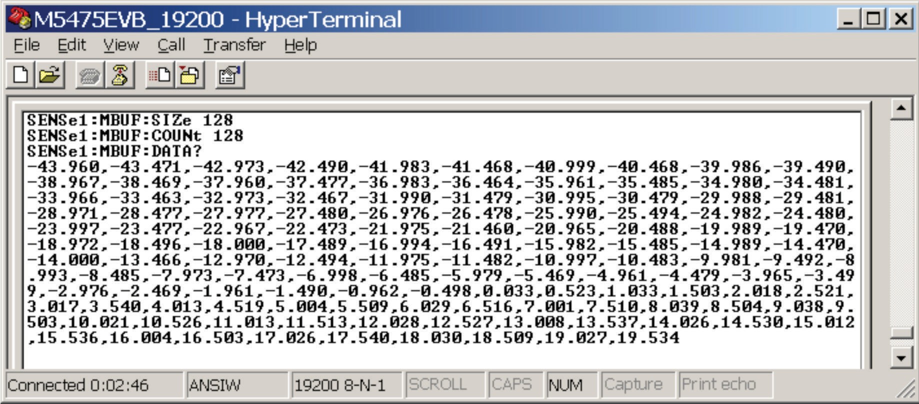
A worked GSM example. A GSM handset is programmed to transmit a power sweep that tests each level of its internal power-control attenuator. The attenuator has 128 levels. Attenuation is incremented for each GSM frame, with the handset transmitting for one timeslot per frame. In GSM, a timeslot is 577 µs and a frame of eight timeslots is 4.615 ms, so the phone transmits a pulsed signal with a 217 Hz period.

The meter is set to trigger on the signal's rising edge for each timeslot, then perform an interval-average power measurement over the active portion (typically the middle 550 µs of the pulse). A trigger holdoff of about 4.5 ms ensures the meter does not retrigger before the next timeslot begins. The trigger level must be low enough that even the lowest pulse amplitude triggers a sweep.

To initiate the sweep, the meter is configured and armed, and the source commanded to begin a sweep of 128 frames. The sweep takes 128 / 217 = 590 ms. At the end, the controller queries the meter to retrieve the buffer containing all 128 readings. If carefully optimized, the entire process should take less than one second.

Buffered measurement modes. Modern power meters acquire a series of measurements into memory with little or no processing. If needed, the data may be post-processed after the acquisition cycle is complete. Buffered acquisition is set up and executed under PC control. Results can be collected in free-run or triggered mode. Data rates of up to 1,000 readings per second are typical for free-run mode; the triggered mode rate may be lower because of latency to re-arm for the next trigger event. Buffer sizes of 1 million readings or more per channel are typical. For buffers implemented as FIFOs (first in, first out), data collection can continue beyond the buffer fill time, since FIFOs can be read while still being filled. Reading the buffer when it is half-filled allows continuous acquisition as read and write pointers update as the FIFO is accessed. This works as long as the time to read a fraction of the buffer is less than the time to fill the entire buffer. Binary data transfer reduces data transfer times further when needed.

For CW mode, up to 1 million readings can be stored at preprogrammed rates as high as 1,000 readings per second. Data is transferred to the host PC after all readings are stored. The user trades off time resolution, measurement duration, and data set size. This mode is best for continuous modulation formats where the power is stepped at periodic intervals.

For pulsed signal types, triggered pulse measurements can also be buffered to record power sweeps for discontinuous formats such as GSM or TDMA. Each pulse trigger stores a reading in the buffer. The Berkeley Nucleonics 12100 series supports buffered sweep mode out of the box: arm with a single SCPI command, capture up to 1 million triggered readings, return them in a single bulk transfer when the sweep completes.

8.3 Communication Amplifier Testing

For communications PAs, the canonical test is the 1 dB compression point. Sweep input power upward and find the input level at which the output is 1 dB below the linear extrapolation. This defines the amplifier's useful linear range for narrowband CW signals. For modulated signals, the situation is more complex. Statistical analysis using a peak power meter offers a fast way to characterize amplifier behavior under realistic operating conditions.

Part 1. Measure the 1 dB compression point of the DUT. Use a peak sensor on both input and output. Sweep input power from well below compression to well above. Plot output versus input in dB. Find the point where output deviates 1 dB from the linear fit. That is your P1dB.

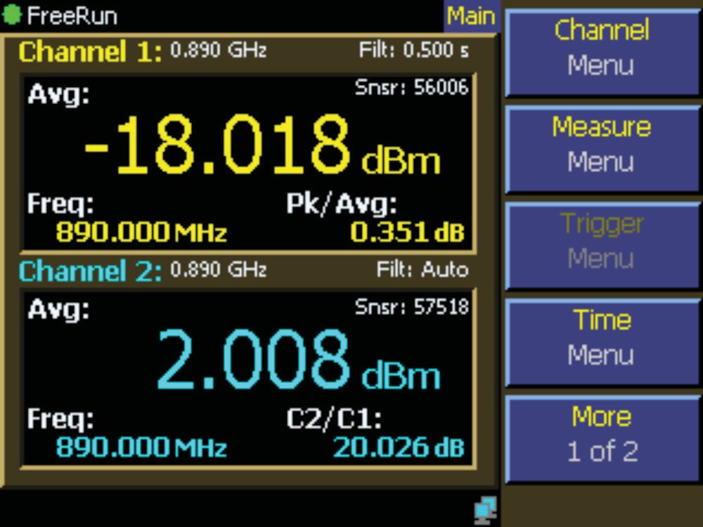
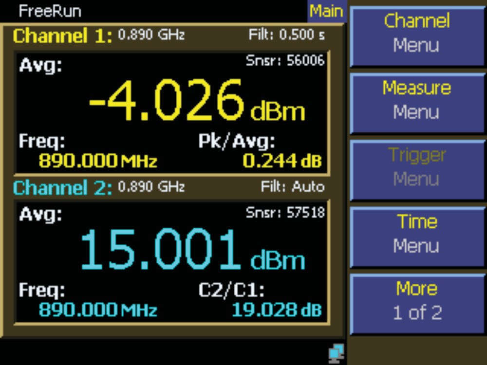
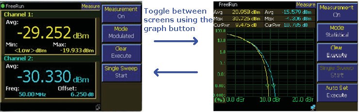
A two-channel power meter with buffered sweep makes this measurement in seconds. The signal generator is programmed to step the input power, the meter is armed in buffered triggered mode, and at the end the controller pulls back the full input-vs-output table. At a small-signal drive level the gain (the Channel 2 to Channel 1 ratio) reads about 20 dB. As the input is raised toward compression, the gain drops by 1 dB, and the output power at that point is the P1dB figure-of-merit for the amplifier.

Part 2. Characterize performance around P1dB using statistical analysis. For amplifiers driven by modulated signals, the 1 dB compression point is only a rough indicator. The real question is how much of the signal's statistical distribution enters compression. A good crest-factor reduction (CFR) algorithm can allow operation well above P1dB on a CCDF basis, improving amplifier efficiency substantially.

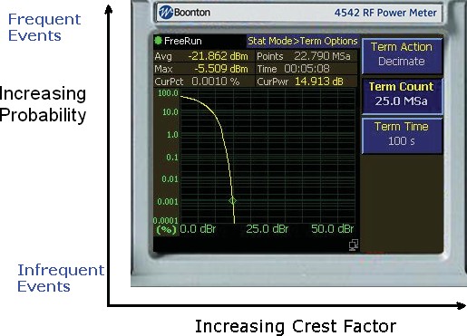
The statistical view is the complementary cumulative distribution function, or CCDF. It plots the probability that the signal exceeds a given level above its average, with crest factor increasing along the horizontal axis and probability falling along the vertical axis. Frequent low-crest events sit toward the upper left, infrequent high-crest peaks toward the lower right. A meaningful statistical measurement needs a large number of samples, and Berkeley Nucleonics power meters can collect millions of peak power readings in seconds.

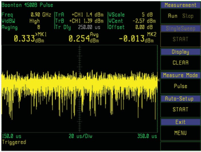
Drive the amplifier with the actual modulated signal it will see in service. A CDMA or similar spread-spectrum waveform looks noise-like in the time domain, with large peaks riding on a much lower average, so the time-domain trace alone says little about how often those peaks occur.

Capture CCDFs at the input and output simultaneously. The shape difference between input and output reveals exactly how the amplifier compresses across the statistical distribution of the input signal. This is far more informative than P1dB alone, and it correlates more directly with system-level performance metrics such as ACLR and EVM.

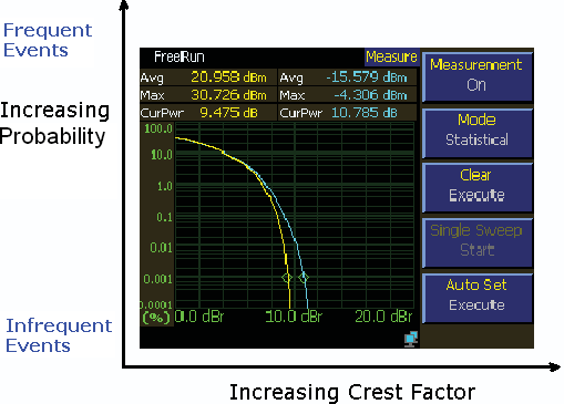
On a two-channel peak power meter the numeric two-channel view and the statistical CCDF view are toggled with the graph button, so the same setup gives both the gain reading and the distribution.

Part 3. Verify across modulation and temperature. Amplifier performance drifts with temperature and with modulation type. Run the full sweep at cold, room, and hot temperatures, and at every modulation format the amplifier is intended to support. Store results in a traceable database. Your QA team will thank you. Your field-failure analysis team will thank you more.

Engineer's corner. A common production-line shortcut is to measure CCDF at one frequency, one temperature, and one modulation format, then declare the amplifier characterized. Skip that shortcut. Run the full matrix at least once during NPI, save the data, and use it as the gold reference against which production units are compared. The Berkeley Nucleonics 12100 series, with its built-in real-time clock and large internal logging buffer, makes building that gold reference dataset straightforward.